Gaussian filter

What is a Gaussian Filter?

In image processing, a Gaussian filter is a type of smoothing filter used to reduce noise in an image.

It performs filtering by convolving an image with a kernel that approximates a Gaussian distribution.

2D Gaussian Distribution

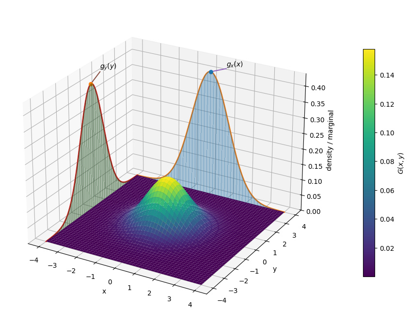
For Gaussian filtering in images, a 2D Gaussian distribution is used.

Typically, in the absence of special considerations, we assume that the x and y directions are independent and follow the same variance.

This means we don’t need to consider general Gaussian distributions with correlations between x and y or different variances.

First, let’s display the probability density function of such a 2D Gaussian distribution.

The marginal distribution in the x-direction is a 1D Gaussian distribution with standard deviation σ:

$$g_x(x)=\frac{1}{\sqrt{2\pi {\sigma }^2}}\exp (-\frac{x^2}{2{\sigma }^2})$$

Similarly, the marginal distribution in the y-direction is a 1D Gaussian distribution with standard deviation σ:

$$g_y(y)=\frac{1}{\sqrt{2\pi {\sigma }^2}}\exp (-\frac{y^2}{2{\sigma }^2})$$

Since these are independent, the joint probability density function is:

$$G(x,y)=g_x(x)g_y(y)=\frac{1}{2\pi {\sigma }^2}\exp (-\frac{x^2+y^2}{2{\sigma }^2})$$

Approximation of 2D Gaussian Distribution

This distribution $G(x,y)$ extends infinitely.

Since convolving an image (which consists of finite, discrete pixels) with something that extends infinitely is difficult, $G(x,y)$ is approximated by a finite, discrete grid with odd dimensions.

This grid is the kernel.

A common example of such a kernel is shown below.

How is this kernel approximated from $G(x,y)$?

In practice, the kernel is computed by evaluating $G(x,y)$ at each grid point and then normalizing so that the sum of all kernel values equals 1.

For instance, in the case of a 3x3 grid with $\sigma =0.85$, we have:

$$G(0,0)=\frac{1}{2\pi {\sigma }^2}\exp (-\frac{0}{2{\sigma }^2})=\frac{1}{2\pi {\sigma }^2}\fallingdotseq 0.22$$

$$G(1,0)=G(-1,0)=G(0,1)=G(0,-1)=\frac{1}{2\pi {\sigma }^2}\exp (-\frac{1}{2{\sigma }^2})\fallingdotseq 0.11$$

$$G(1,1)=G(-1,1)=G(1,-1)=G(-1,-1)=\frac{1}{2\pi {\sigma }^2}\exp (-\frac{2}{2{\sigma }^2})\fallingdotseq 0.055$$

Summing these values gives:

$$S=\sum _{-1\le x\le 1,-1\le y\le 1}G(x,y)=0.22+0.11\cdot 4+0.055\cdot 4=0.88$$

So, the values of the kernel at each grid point are:

$$K(0,0)=\frac{G(0,0)}{S}=\frac{0.22}{0.88}=\frac{4}{16}$$

$$K(1,0)=K(-1,0)=K(0,1)=K(0,-1)=\frac{G(1,0)}{S}=\frac{0.11}{0.88}=\frac{2}{16}$$

$$K(1,1)=K(-1,1)=K(1,-1)=K(-1,-1)=\frac{G(1,1)}{S}=\frac{0.055}{0.88}=\frac{1}{16}$$

After calculating $G(x,y)$, normalization is required, so the factor $\frac{1}{2\pi {\sigma }^2}$ can be omitted.

If we denote this by $G^{\prime }(x,y)$, we have:

$$G^{\prime }(x,y)=\exp (-\frac{x^2+y^2}{2{\sigma }^2})$$

Also,

$$r=\exp (-\frac{1}{2{\sigma }^2})$$

Then,

$$G^{\prime }(x,y)=r^{x^2+y^2}$$

Thus, to compute the kernel, determine $r$ from $\sigma$, and then write the grid with $r$ raised to the square of the distance from the center.

Normalizing this yields the kernel.

Conversely, if a kernel is given, you can determine the base Gaussian distribution’s $\sigma$ by taking the ratio of the center value to the value of a neighboring grid point, denoting this ratio as $r$:

$$\sigma =\sqrt{-\frac{1}{2\log r}}$$

For example, for the 5x5 grid shown above:

$$r=\frac{\frac{24}{256}}{\frac{36}{256}}=\frac{24}{36}=\frac{2}{3}$$

So,

$$\sigma =\sqrt{-\frac{1}{2\log r}}=\sqrt{-\frac{1}{2\log \frac{2}{3}}}\fallingdotseq 1.11$$

Based on this discussion, an example code to compute a Gaussian filter kernel using numpy is:

import numpy as np


def make_gaussian_kernel(width: int, height: int, sigma: float) -> np.ndarray
    # Ratio of the value at the center to one neighbor
    r = np.exp(-1 / (2 * sigma**2))

    # Center index of the kernel
    mw = width // 2
    mh = height // 2

    # Array of coordinates relative to the center of the kernel
    xs = np.arange(-mw, mw + 1)
    ys = np.arange(-mh, mh + 1)
    x, y = np.meshgrid(xs, ys)

    # Calculate the base array by raising r to the squared distance
    g = r**(x**2 + y**2)

    # Normalize the kernel
    return g / np.sum(g)

Convolution

The resulting kernel is then convolved with the original image to apply the Gaussian filter.

Convolution can be thought of as “integrating the surrounding pixel values according to the kernel.”

Let $I(x,y)$ be the pixel value of the original image and $K(x,y)$ be the kernel. The pixel value $J(x,y)$ of the output image is given by:

$$J(x,y)=K\ast I=\sum _{u=-w}^w\sum _{v=-h}^{h}K(u,v)I(x+u,y+v)$$

where $w$ is half the width of the kernel and $h$ is half the height of the kernel.

Around each point, we compute the inner product with the kernel by multiplying element-wise and summing.

When performing convolution, several variations for handling the edges of the original image can be considered.

For instance, the scipy library’s convolve2d function provides several modes:

https://docs.scipy.org/doc/scipy/reference/generated/scipy.signal.convolve2d.html

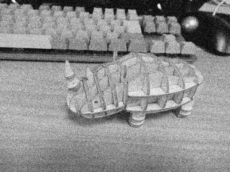
Filter Example

The following shows an example of applying a 3x3 Gaussian filter with $\sigma =0.85$.

It can be observed that the original image is smoothed.

Edges are also blurred, so choosing the appropriate filter depends on the nature of the noise.

Original Image

Filtered Image