Expected Value of the Cosine of a Random Variable Following the Standard Normal Distribution

Proposition

For a random variable $X$ following the standard normal distribution $N(0,1)$, the expected value of $\cos X$ is $\frac{1}{\sqrt{e}}$.

Proof 1

The probability density function of the standard normal distribution is given by:

$$f(x)=\frac{1}{\sqrt{2\pi }}\exp [-\frac{x^2}{2}]$$

Therefore, the expectation of $\cos X$ is:

$$E[\cos X]={\int }_{-\mathrm{\infty }}^{\mathrm{\infty }}\cos x\cdot f(x)dx={\int }_{-\mathrm{\infty }}^{\mathrm{\infty }}\cos x\frac{1}{\sqrt{2\pi }}\exp [-\frac{x^2}{2}]dx$$

To compute this integral, we use the fact that:

$$\cos x=\frac{e^{ix}+e^{-ix}}{2}$$

Thus:

$$E[\cos X]=\frac{1}{2\sqrt{2\pi }}{\int }_{-\mathrm{\infty }}^{\mathrm{\infty }}\exp [-\frac{x^2}{2}+ix]dx+\frac{1}{2\sqrt{2\pi }}{\int }_{-\mathrm{\infty }}^{\mathrm{\infty }}\exp [-\frac{x^2}{2}-ix]dx$$

By substituting $t=-x$, it is shown that the first and second terms on the right-hand side are equal.

Therefore:

$$E[\cos X]=\frac{1}{\sqrt{2\pi }}{\int }_{-\mathrm{\infty }}^{\mathrm{\infty }}\exp [-\frac{x^2}{2}-ix]dx$$

To solve this, complete the square in the exponent of the integrand:

$$E[\cos X]=\frac{1}{\sqrt{2\pi }}{\int }_{-\mathrm{\infty }}^{\mathrm{\infty }}\exp [-\frac{(x+i{)}^2}{2}-\frac{1}{2}]dx=\frac{1}{\sqrt{e}\cdot \sqrt{2\pi }}{\int }_{-\mathrm{\infty }}^{\mathrm{\infty }}\exp [-\frac{(x+i{)}^2}{2}]dx$$

Substitute $z=x+i$:

$$E[\cos X]=\frac{1}{\sqrt{e}\cdot \sqrt{2\pi }}{\int }_{i-\mathrm{\infty }}^{i+\mathrm{\infty }}\exp [-\frac{z^2}{2}]dz$$

This becomes a complex integral.

Consider a rectangular contour $C$ with vertices $-R,-R+i,R+i,R$:

$$C_1:-R\to -R+i$$

$$C_2:-R+i\to R+i$$

$$C_3:R+i\to R$$

$$C_4:R\to -R$$

$$C:C_1+C_2+C_3+C_4$$

Since $C$ is a simple closed curve and $\exp [-\frac{z^2}{2}]$ is analytic, by Cauchy’s integral theorem:

$${\int }_C\exp [-\frac{z^2}{2}]dz=0$$

Also, assuming $R$ is large enough,

$$|{\int }_{C_1}\exp [-\frac{z^2}{2}]dz|=|{\int }_0^1\exp [-\frac{(-R+it{)}^2}{2}]dt|\le {\int }_0^1|\exp [-\frac{(-R+it{)}^2}{2}]|dt={\int }_0^1\exp [-\mathrm{\Re }\frac{(-R+it{)}^2}{2}]dt={\int }_0^1\exp [-\frac{R^2-t^2}{2}]dt\le {\int }_0^1\exp [-\frac{R^2-1}{2}]dt=\exp [-\frac{R^2-1}{2}]$$

Thus, as $R\to \mathrm{\infty }$,

$${\int }_{C_1}\exp [-\frac{z^2}{2}]dz\to 0$$

Similarly,:

$${\int }_{C_3}\exp [-\frac{z^2}{2}]dz\to 0$$

Therefore, as $R\to \mathrm{\infty }$:

$${\int }_{C_2}\exp [-\frac{z^2}{2}]dz+{\int }_{C_4}\exp [-\frac{z^2}{2}]dz\to 0$$

The integral along $C_4$ is the Gaussian integral along the real axis:

$${\int }_{C_4}\exp [-\frac{z^2}{2}]dz\to -\sqrt{2\pi }$$

Thus:

$${\int }_{C_2}\exp [-\frac{z^2}{2}]dz\to \sqrt{2\pi }$$

Hence:

$$E[\cos X]=\frac{1}{\sqrt{e}\cdot \sqrt{2\pi }}{\int }_{i-\mathrm{\infty }}^{i+\mathrm{\infty }}\exp [-\frac{z^2}{2}]dz=\frac{1}{\sqrt{e}\cdot \sqrt{2\pi }}\underset{R\to \mathrm{\infty }}{lim}{\int }_{C_2}\exp [-\frac{z^2}{2}]dz=\frac{1}{\sqrt{e}\cdot \sqrt{2\pi }}\sqrt{2\pi }=\frac{1}{\sqrt{e}}$$

Proof 2

Using the Maclaurin series expansion of $\cos x$:

$$E[\cos X]=E[(1-\frac{X^2}{2!}+\frac{X^4}{4!}-\dots )]=E[1]-\frac{E[X^2]}{2!}+\frac{E[X^4]}{4!}-\dots$$

Let:

$$I_n:=E[X^{2n}]={\int }_{-\mathrm{\infty }}^{\mathrm{\infty }}{x}^{2n}\frac{1}{\sqrt{2\pi }}{e}^{\frac{-x^2}{2}}dx$$

Using integration by parts:

$${\int }_{-\mathrm{\infty }}^{\mathrm{\infty }}{x}^{2n}{e}^{\frac{-x^2}{2}}dx={\left[\frac{x^{2n+1}}{2n+1}{e}^{\frac{-x^2}{2}}\right]}_{-\mathrm{\infty }}^{\mathrm{\infty }}-{\int }_{-\mathrm{\infty }}^{\mathrm{\infty }}\frac{x^{2n+1}}{2n+1}\cdot (-x)e^{\frac{-x^2}{2}}dx=0+{\int }_{-\mathrm{\infty }}^{\mathrm{\infty }}\frac{x^{2n+2}}{2n+1}{e}^{\frac{-x^2}{2}}dx=\frac{1}{2n+1}{\int }_{-\mathrm{\infty }}^{\mathrm{\infty }}{x}^{2n+2}{e}^{\frac{-x^2}{2}}dx$$

So:

$$I_{n+1}=(2n+1)I_n$$

Using this recurrence relation repeatedly:

$$I_n=(2n-1)!!I_0=(2n-1)!!$$

Thus:

$$E[\cos X]=I_0-\frac{I_1}{2!}+\frac{I_2}{4!}-\dots =1-\frac{1!!}{2!}+\frac{3!!}{4!}-\dots =1-\frac{1}{2\cdot 1}+\frac{3\cdot 1}{4\cdot 3\cdot 2\cdot 1}-\dots =1-\frac{1}{2}+\frac{1}{4\cdot 2}-\dots =1-\frac{1}{2}\cdot \frac{1}{1!}+\frac{1}{2^2}\cdot \frac{1}{2!}-\dots =\sum _{n=0}^{\mathrm{\infty }}\frac{(-\frac{1}{2}{)}^n}{n!}=e^{-\frac{1}{2}}=\frac{1}{\sqrt{e}}$$

Note

It should be noted that the expected value of $\sin X$ is trivial and equals $0$. This is because the integrand becomes the product of an even function and an odd function.

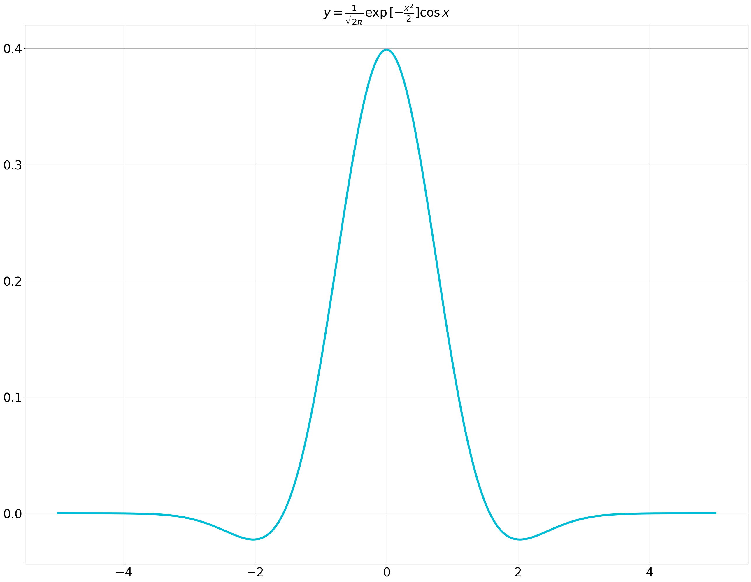
The graph of the integrand function considered here is as follows. In this case, we calculated the area (considering the sign) of the region enclosed by this graph and the x-axis.

If the characteristic function of the normal distribution is known, this problem is very simple.

Since the probability density function is an even function,

$$\varphi (t)=E[e^{itX}]=E[\cos (tX)]$$

therefore, by substituting $t=1$ into the characteristic function

$$\varphi (t)=\exp [-\frac{t^2}{2}]$$

the result can be immediately obtained.

Fourier Transform of the Probability Density Function of the Normal Distribution (Gaussian Function)