How to Use FFT (NumPy, SciPy)
What is FFT?
One of the fundamental tools in signal processing is FFT.
FFT stands for Fast Fourier Transform, an algorithm for quickly computing the Discrete Fourier Transform (DFT).
Using FFT
The FFT algorithm is highly efficient due to its use of symmetry, which is fascinating in itself, but here we will focus on how to use it rather than explaining the principles.
Fourier Transform is often described as “a conversion from the time domain to the frequency domain.”
Let’s see how this works in practice.
In this case, we will apply FFT to audio signals, which are easier to understand because we can hear them.
FFT in NumPy
FFT is often provided by libraries, which is convenient because it’s optimized for speed.
Implementing it yourself can be fun, but using pre-optimized versions is easier.
Here, we will use the FFT implementation from the NumPy library in Python.
https://numpy.org/doc/stable/reference/routines.fft.html
NumPy’s FFT includes the following functions:
- Standard FFTs
- fft
- ifft
- fft2
- ifft2
- fftn
- ifftn
- Real FFTs
- rfft
- irfft
- rfft2
- irfft2
- rfftn
- irfftn
- Hermitian FFTs
- hfft
- ihfft
- Helper routines
- fftfreq
- rfftfreq
- fftshift
- ifftshift
There are functions for complex input signals like fft and for real input signals like rfft, as well as inverse Fourier transforms like ifft and irfft.
Additionally, there are 2D and N-dimensional variants: fft2, rfft2, ifft2, irfft2, fftn, rfftn, ifftn, irfftn.
Furthermore, for complex input signals with Hermitian symmetry, hfft and its inverse ihfft are available.
Helper routines like fftfreq and rfftfreq are used to obtain frequency domain samples from fft/rfft results.
For a signal with a sampling frequency
Notice that the denominator starts at
This structure is similar to interpreting binary numbers from
fftfreq returns this type of array but is unordered, which can be inconvenient.
To address this, fftshift rearranges it as follows:
ifftshift performs the reverse operation.
Different functions are used for complex and real signals because for real signals, the fft result is symmetric with negative frequency components being the complex conjugate of the corresponding positive frequencies, which allows for faster computation.
The symmetry in fft results for real signals can be understood by revisiting the definition of Fourier transform:
Taking the conjugate of both sides:
This demonstrates that “negative frequency components are the complex conjugates of corresponding positive frequencies.”
Note that this symmetry is called Hermite symmetry.
In practice, many signals are real. For this data, we will use rfft.
rfftfreq returns the following type of array:
The following code behaves the same.
import numpy as np

def my_rfftfreq(n, fs):
    return np.linspace(0, fs / 2, n // 2 + 1)
Note that numpy.fft.rfftfreq takes the sampling interval
For rfft, the result is already sorted in ascending order, so functions like rfftshift are not needed.
The last element of the result from rfftfreq is
According to the sampling theorem, the Nyquist frequency is the upper limit of the signal frequencies that can be reconstructed with a given sampling frequency.
Audio Data 1: 440Hz Sine Wave
The first audio data is a 440Hz sine wave lasting 10 seconds. This corresponds to the pitch A4.
This audio was created with the following code:
import numpy as np
import scipy.io.wavfile as wavfile

# Parameters
fs = 48000  # Sampling rate (Hz)
f = 440.0  # Frequency of sine wave (Hz)
duration = 10.0  # Length of sine wave (seconds)

n_samples = int(fs * duration)

# Create time axis
t = np.linspace(0, duration, n_samples, endpoint=False)

# Generate sine wave
s = np.sin(2 * np.pi * f * t)

# Convert to 16-bit PCM format
s_16bit_pcm = np.int16(s * 32767)

# Write WAV file
wavfile.write("sine_wave.wav", fs, s_16bit_pcm)
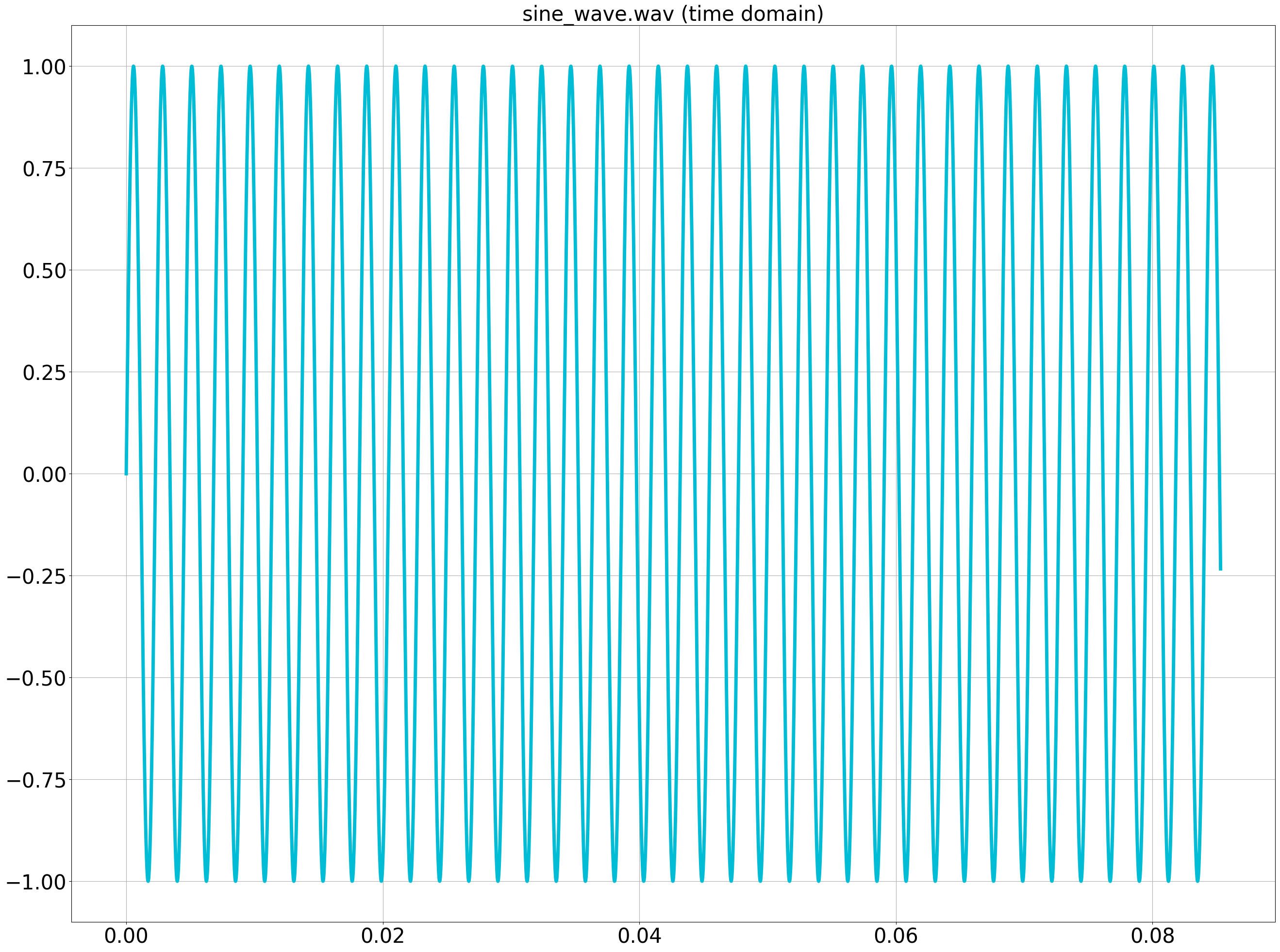
Plotting the first 4096 samples of this signal looks like the following.
Let’s perform FFT on this signal.
Continuing from the previous code, we execute FFT.
# Extract the first 4096 samples
s = s[:4096]

# FFT
z = np.fft.rfft(s)

# Frequencies
f = np.fft.rfftfreq(len(s), 1 / fs)
Plotting f on the x-axis and the magnitude of z on the y-axis gives the frequency domain plot.
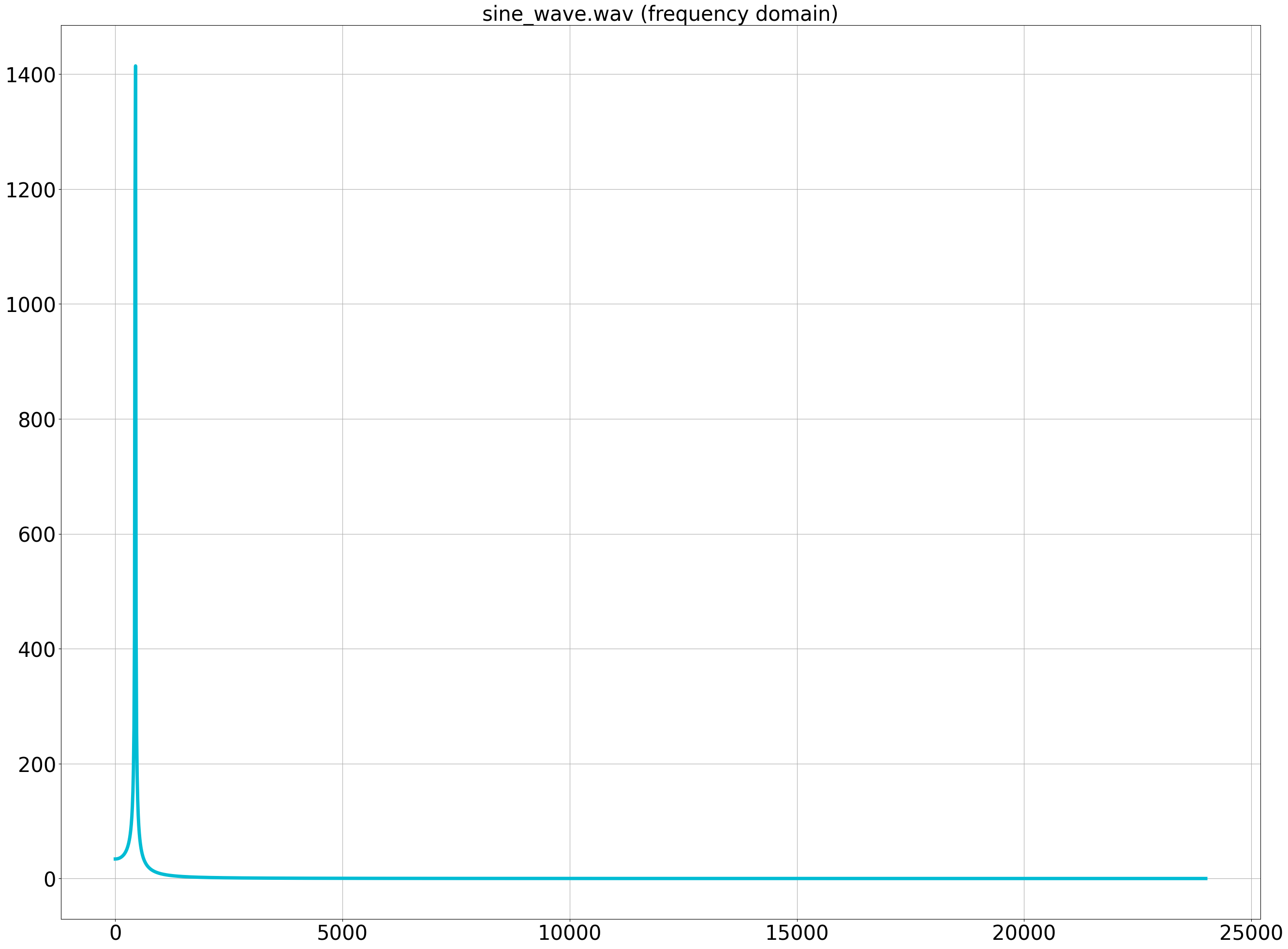
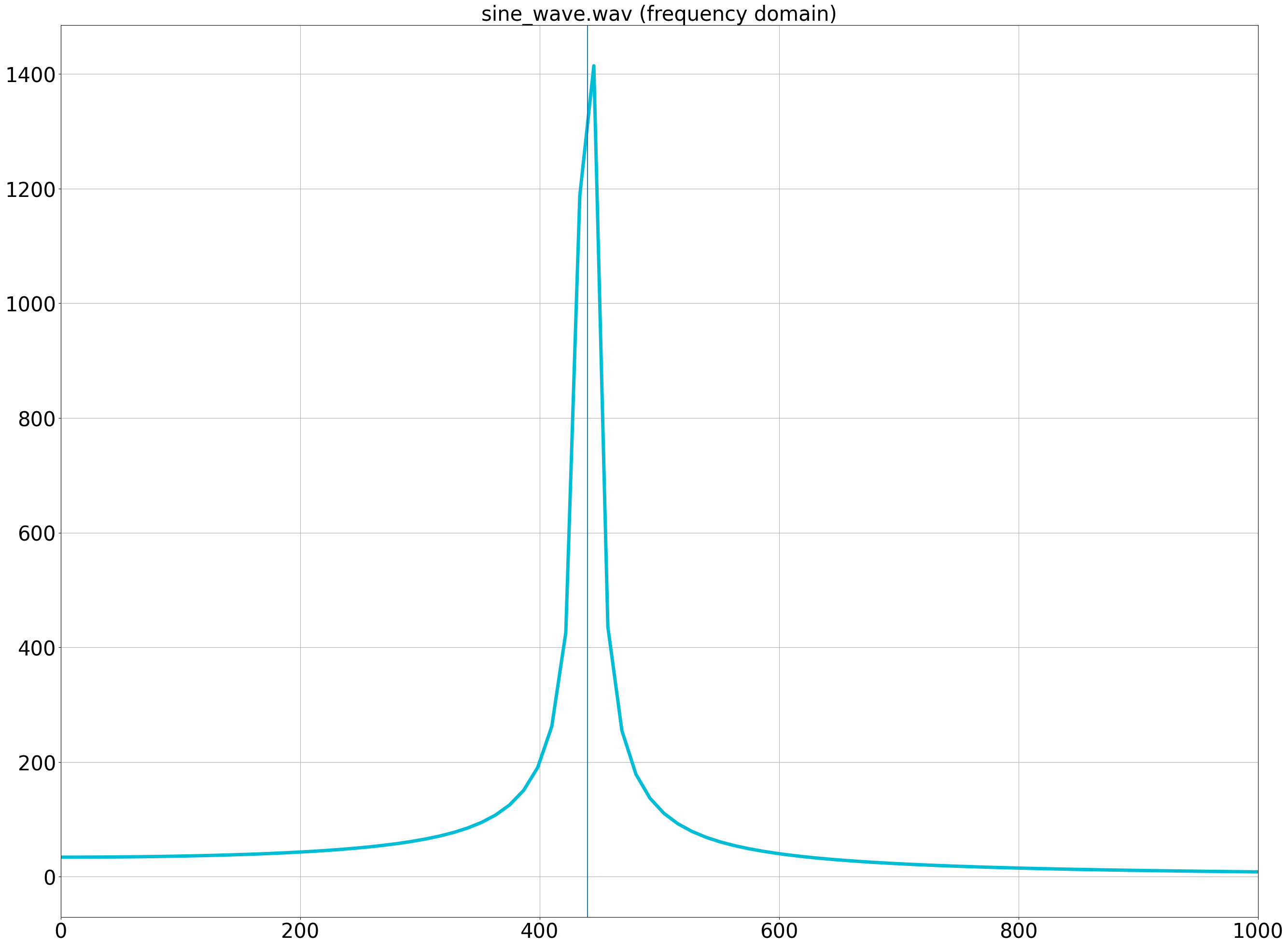
Zooming in around 440Hz, we can confirm a peak at around 440Hz in the input signal.
Audio Data 2: C-F-G-C Cadence
The second audio data is a C-F-G-C cadence.
The differences from Audio Data 1 are:
- It contains multiple frequencies forming chords.
- The chords change over time.
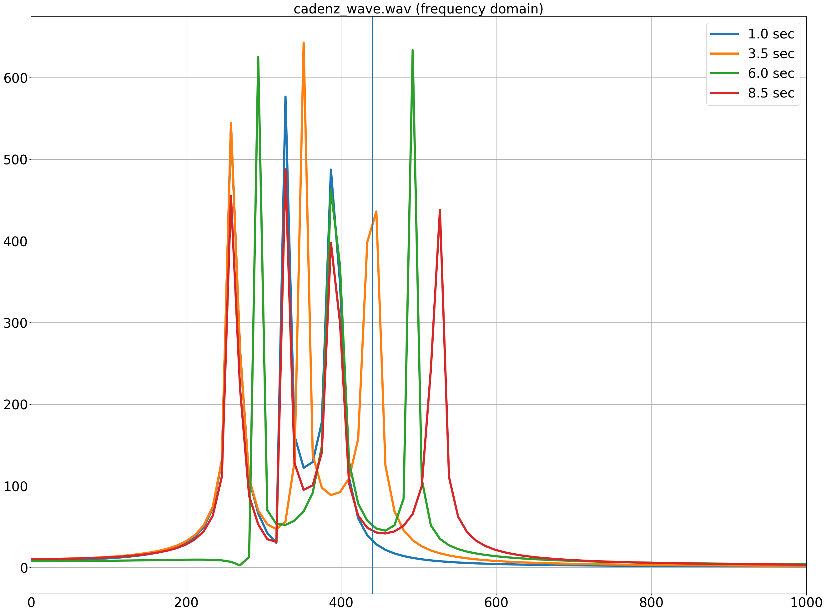
FFT results at 1s, 3.5s, 6s, and 8.5s with a chunk size of 4096 are shown in the following figure.
Each point shows 3 or 4 peaks corresponding to the chord components. The changing peaks indicate the evolving chords over time.
Spectrogram
As seen in Audio Data 2, it is common for sounds to change over time.
Music, for instance, creates melodies through temporal changes in frequency.
While it’s possible to visualize FFT results at different time points with varying colors, this can be hard to interpret for time-varying changes.
Instead, a graph with time on the x-axis and frequency on the y-axis, with intensity represented by color, is more effective.
Such a graph is called a spectrogram and is widely used in acoustics.
SciPy’s STFT
To create a spectrogram, we perform Short-Time Fourier Transform (STFT).
STFT involves dividing the input signal into small chunks (short time intervals) and performing Fourier Transform on each chunk.
In practice, a window function (often a Hann window) is applied to clearly define the time of interest, and chunks are overlapped to make frequency changes as smooth as possible.
Here, we use the ShortTimeFFT class from SciPy’s signal module.
Various window functions are defined in scipy.signal.windows, and we use the Hann window, the most commonly used window function.
The overlap width is set to 3/4 of the chunk width (i.e., hop size is 1/4).
Performing STFT is as follows:
# Hann window
win = signal.windows.hann(4096)

# Short-Time Fourier Transform
SFT = signal.ShortTimeFFT(win, 4096 * 1 // 4, fs)
Sx = SFT.stft(s)
The spectrogram generated following the reference example is shown below.
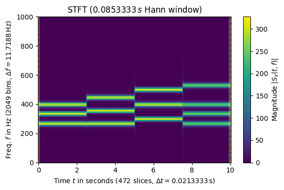
- 0.0s - 2.5s : C-E-G
- 2.5s - 5.0s : C-F-A
- 5.0s - 7.5s : D-G-B
- 7.5s - 10.0s : C-E-G-C
This is evident from the plot.
Audio Data 3: Reading
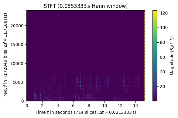
Finally, here is a spectrogram of my own reading voice as an example of human voice.
It is said that the fundamental frequency of an adult male’s voice is around 120Hz - 200Hz, which aligns with the spectrogram peaks.
Additionally, higher frequencies around 7000Hz are present in the voice.
Notably, there are prominent peaks around 5000Hz at approximately 6.5s and 12.5s.
Listening to the original audio, these segments correspond to strong sibilants in the speech.